Accessing cloud-based datasets
R counterpart:
sdp-cloud-data.Rmd— the Python version below mirrors its structure.
The RMBL Spatial Data Platform hosts >100 curated raster products on S3 as cloud-optimized GeoTIFFs. pysdp lets you find, open, and work with these rasters without downloading the full files. This guide walks the basics.
Setup
Finding datasets
Get a DataFrame of the full catalog:
Narrow with filters:
For advanced filtering, work with the DataFrame directly — any pandas operation is fair game:
snow = cat[cat["Product"].str.contains("Snow", case=False)]
snow[["CatalogID", "Product", "TimeSeriesType"]]
The CatalogID column is pySDP's canonical handle for each product. R4D001, for example, identifies the annual snow persistence time-series for the Upper Gunnison domain.
Detailed metadata
Beyond the catalog DataFrame, each product has a companion XML metadata document describing provenance, sensors, processing history, etc.:
Visualizing SDP domains
The four SDP domains (UG, UER, GT, GMUG) are small enough to plot together. Their boundary polygons are hosted alongside the raster products:
domains = [
    ("UG",   "Upper Gunnison",         "https://rmbl-sdp.s3.us-east-2.amazonaws.com/data_products/supplemental/UG_region_vect_1m.geojson"),
    ("UER",  "Upper East River",       "https://rmbl-sdp.s3.us-east-2.amazonaws.com/data_products/supplemental/UER_region_vect_1m.geojson"),
    ("GT",   "Gothic Townsite",        "https://rmbl-sdp.s3.us-east-2.amazonaws.com/data_products/supplemental/GT_region_vect_1m.geojson"),
]

import pandas as pd
frames = [gpd.read_file(u).assign(Domain=name) for _, name, u in domains]
bounds = pd.concat(frames).pipe(gpd.GeoDataFrame, crs=frames[0].crs)
bounds.explore(column="Domain", tiles="Esri.NatGeoWorldMap", alpha=0.6)
GeoDataFrame.explore() produces a folium-backed interactive map — the geopandas analog of terra::plet() in rSDP:
Connecting to data in the cloud
open_raster() returns an xarray.Dataset backed by a lazy COG read — no data is transferred until you .compute(), .plot(), or slice it.
Single-layer products
Inspect the structure: dimensions, resolution, CRS (EPSG:32613), and data variable name. A quick plot:
import matplotlib.pyplot as plt
ug_elev[next(iter(ug_elev.data_vars))].plot.imshow(cmap="terrain", robust=True)
plt.gca().set_aspect("equal")
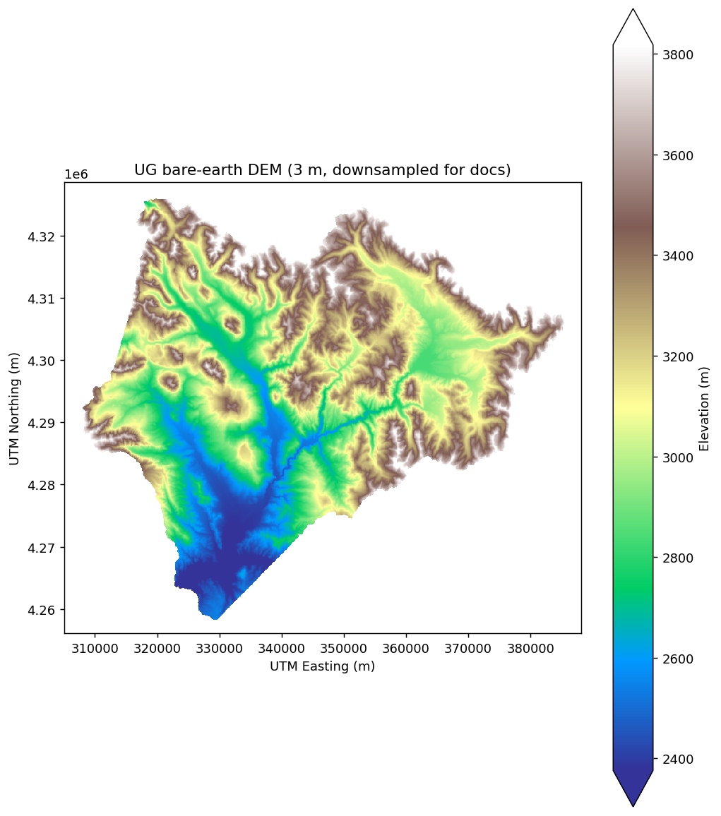
(The DEM here is downsampled by a factor of 60 for fast rendering in the docs; the full 3 m resolution is ~584 million cells and about 1 GB per read.)
Cropping to an area of interest only fetches the portion of the COG that intersects the bounding box:
gt_bounds = bounds[bounds["Domain"] == "Gothic Townsite"].to_crs(ug_elev.rio.crs)
gt_elev = ug_elev.rio.clip(gt_bounds.geometry, from_disk=True)
gt_elev
from_disk=True streams the crop directly from the COG via GDAL's windowed reads. Without it, rioxarray materializes the full raster first and then crops, which defeats the cloud-native access model.
Time-series products
Many SDP products are daily, monthly, or annual time-series. Pass years= (for Yearly products), months= (Monthly), or date_start / date_end (any type) to slice the time dimension at open-time:
snow_years = pysdp.open_raster("R4D001", years=[2018, 2019, 2020])
snow_years.sizes   # {'time': 3, 'y': ..., 'x': ...}
Check the catalog's MinYear / MaxYear / MinDate / MaxDate fields to see what's available:
ts = cat[cat["TimeSeriesType"].isin(["Yearly", "Monthly", "Daily"])]
ts[["CatalogID", "Product", "TimeSeriesType", "MinDate", "MaxDate", "MinYear", "MaxYear"]]
When to download data locally
Lazy cloud reads are ergonomic but have a cost — every data access triggers an HTTP range request. For operations that touch many cells (random sampling, whole-raster reductions, repeated algebra), local access is substantially faster.
# 100-point random sample on a cloud-hosted snow time-series:
import time
t0 = time.time()
sample = snow_years.stack(pix=("y", "x")).isel(pix=slice(0, 100)).compute()
print(f"cloud sample: {time.time() - t0:.1f}s")
Use pysdp.download() to mirror to disk when needed:
Then open from disk with rioxarray.open_rasterio(...), or via the packaged CSV's Data.URL pointing at the local copy.
Operations that benefit most from local storage:
- Whole-raster reductions (mean, std over all cells)
- Resampling or reprojection (touches every pixel)
- Repeated extractions from the same product
For narrow operations — cropping to a small AOI, extracting at a handful of points — cloud reads are usually fast enough and save the download step.
Next steps
- Wrangling raster data — masking, reprojection, resampling, export
- Field-site sampling — extraction at points and polygons
- Pretty maps — static + interactive visualization