Pretty maps
R counterpart:
pretty-maps.Rmd.
pysdp doesn't ship its own plotting layer — it returns xarray.Dataset and geopandas.GeoDataFrame objects that compose with the rest of the PyData viz ecosystem. This guide covers the three common paths:
- Static maps with
matplotlib+xarray.plot(for papers, reports) - Interactive web maps with
folium/GeoDataFrame.explore()(for exploration, notebooks) - Publication-quality faceted figures with
matplotlibsubplots orhvplot
Setup
Loading data
# Digital elevation model — the base layer for most maps
dem = pysdp.open_raster("R3D009", chunks=None)  # UG 3 m bare-earth DEM

# Vector overlays — load any GeoJSON / GPKG / Shapefile with geopandas
bounds = gpd.read_file(
    "https://rmbl-sdp.s3.us-east-2.amazonaws.com/data_products/supplemental/UG_region_vect_1m.geojson"
)
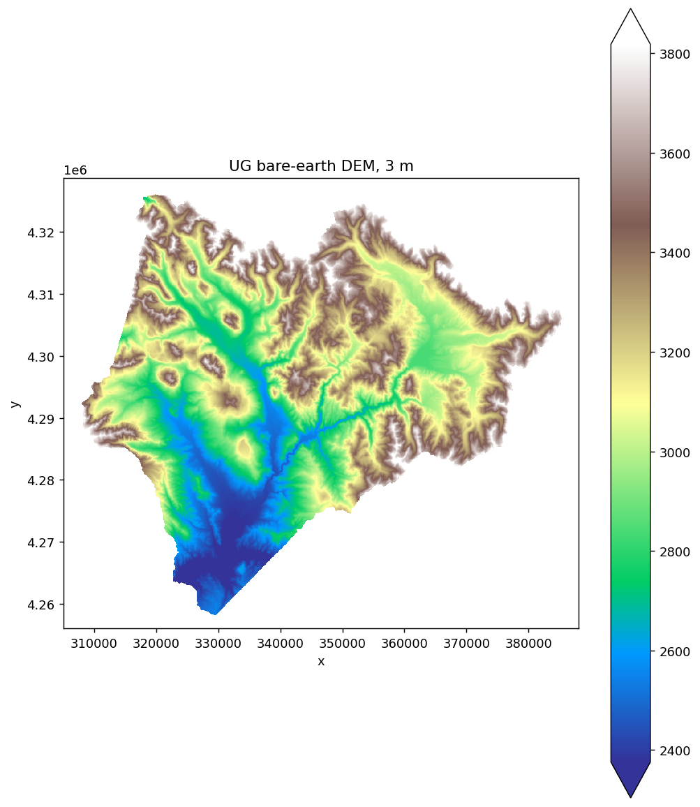
Basic raster map with matplotlib
fig, ax = plt.subplots(figsize=(8, 9))
dem[next(iter(dem.data_vars))].plot.imshow(ax=ax, cmap="terrain", robust=True)
ax.set_aspect("equal")
ax.set_title("UG bare-earth DEM (3 m)")
plt.tight_layout()
.plot.imshow() is xarray's matplotlib wrapper — it handles colorbars, axis labels, and CRS-aware extent automatically. robust=True clips extreme outliers so the colormap stays useful.
Tip: at full resolution the 3 m DEM is ~584 M cells, which is too much to plot directly. Downsample first with dem.coarsen(x=60, y=60, boundary="trim").mean() (or pre-crop to your AOI) before plotting.
Web maps with folium
For exploration in a notebook, GeoDataFrame.explore() gives you a pan/zoom map with a single call:
import folium
m = bounds.explore(column="Domain", tiles="Esri.WorldImagery", cmap="Set2")
for _, row in sites.iterrows():
    folium.Marker(
        location=[row.geometry.y, row.geometry.x],
        popup=row["site"],
        icon=folium.Icon(color="red", icon="star"),
    ).add_to(m)
m
To overlay a raster on a folium map, use folium.raster_layers.ImageOverlay with an RGBA PNG you've rendered from the xarray data. That's more setup — for quick visual checks, xarray.plot + matplotlib is usually faster.
Faceted multi-panel maps
Showing multiple years of a time-series product side-by-side:
snow = pysdp.open_raster("R4D001", years=[2018, 2019, 2020], chunks=None)

fig = snow["UG_snow_persistence_27m_v1"].plot.imshow(
    col="time", col_wrap=3,
    cmap="Blues", robust=True,
    figsize=(14, 5),
)
xarray auto-creates the subplot grid from the col="time" faceting argument.
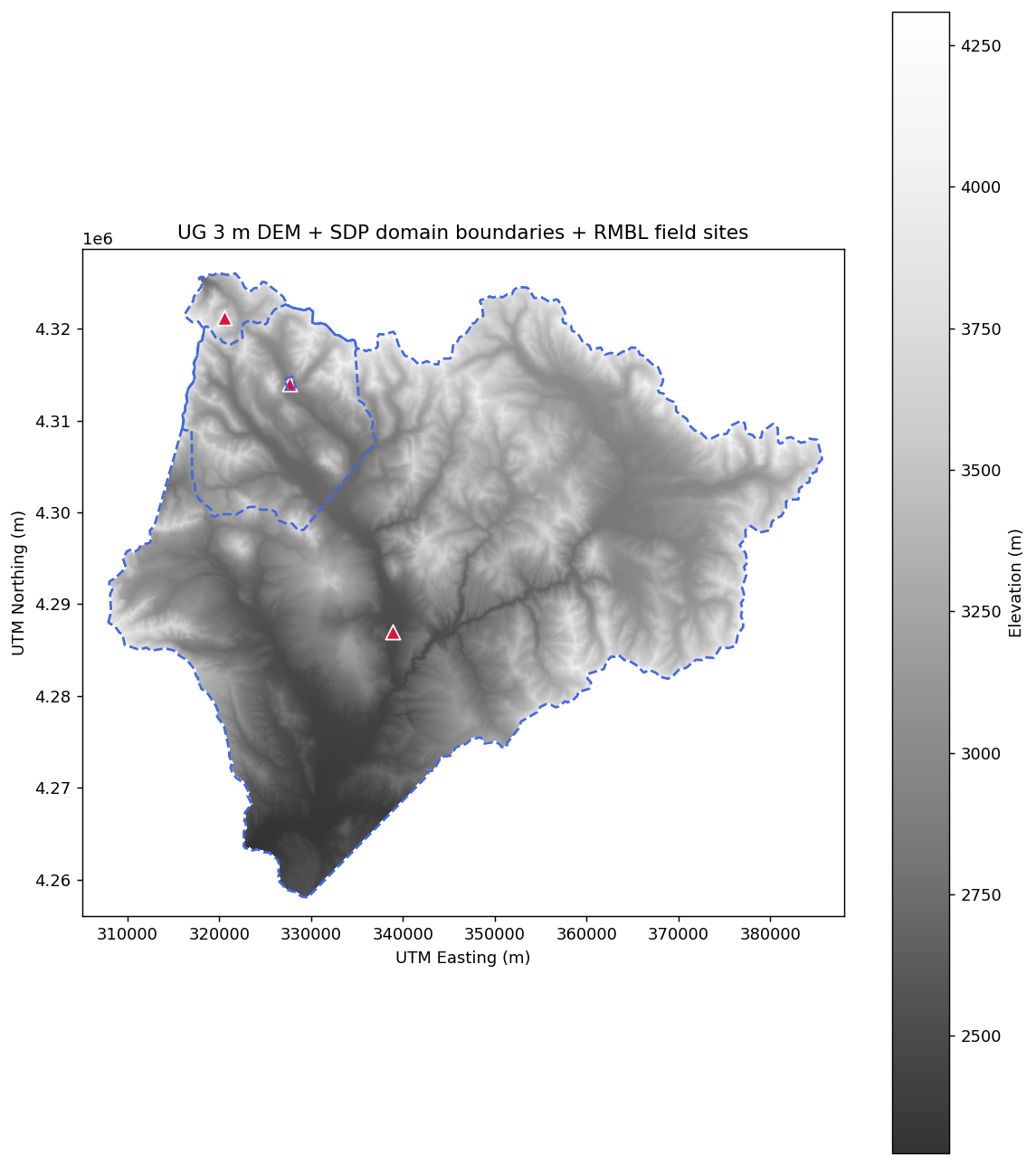
Adding overlays
Combine raster + vector on one figure:
fig, ax = plt.subplots(figsize=(10, 8))

# Base: DEM in grey
dem[next(iter(dem.data_vars))].plot.imshow(
    ax=ax, cmap="Greys_r", add_colorbar=True, alpha=0.8,
)

# Overlay: domain boundaries in the raster's CRS
bounds.to_crs(dem.rio.crs).boundary.plot(
    ax=ax, color="royalblue", linewidth=1.5, linestyle="--",
)

# Overlay: field sites
from shapely.geometry import Point
sites = gpd.GeoDataFrame(
    {"site": ["Roaring Judy", "Gothic", "Galena Lake"]},
    geometry=[
        Point(-106.853186, 38.716995),
        Point(-106.988934, 38.958446),
        Point(-107.072569, 39.021644),
    ],
    crs="EPSG:4326",
).to_crs(dem.rio.crs)
sites.plot(ax=ax, color="crimson", markersize=80, marker="^", edgecolor="white")

ax.set_title("UG 3 m DEM + SDP domain boundaries + RMBL field sites")
ax.set_aspect("equal")
plt.tight_layout()
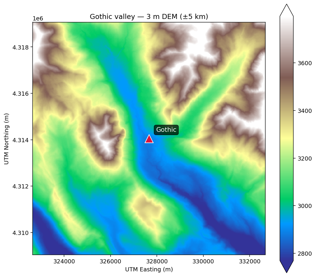
Zooming in
Crop to an AOI before plotting for faster rendering and sharper detail:
# 5 km buffer around Gothic, in UTM 13N
gothic_utm = sites.iloc[[1]].geometry.iloc[0]
buffer = 5_000
clipped = dem[next(iter(dem.data_vars))].rio.clip_box(
    gothic_utm.x - buffer, gothic_utm.y - buffer,
    gothic_utm.x + buffer, gothic_utm.y + buffer,
)

fig, ax = plt.subplots(figsize=(8, 7))
clipped.plot.imshow(ax=ax, cmap="terrain", robust=True)
ax.set_title("Gothic valley — 3 m DEM (±5 km)")
ax.set_aspect("equal")
Exporting
PNG (for web, reports):
PDF (for publication):
GeoTIFF of a styled map isn't straightforward with matplotlib — if you need a georeferenced map image for GIS, write the raster directly with rio.to_raster and restyle downstream.
Alternatives worth knowing
hvplot— interactive notebook plots via holoviews:dem.hvplot.image(x="x", y="y"). Nice for lots of zooming.lonboard— GPU-accelerated map rendering for large vector datasets; excellent for 100k+ point displays.leafmap— folium/ipyleaflet wrapper with sensible defaults for Earth-observation workflows; supports COG display directly.
For static publication figures, matplotlib + xarray.plot remains the most-used path.
Next steps
- Field-site sampling — generating the extracted data that your maps visualize
- API reference for pySDP's full function surface