Sampling SDP Data Products at Field Sites
Source:vignettes/field-site-sampling.Rmd
field-site-sampling.Rmdby Ian Breckheimer, updated 21 March 2023.
Data products generated as part of the RMBL Spatial Data Platform are meant to provide important environmental context for measurements collected in the field. Taking advantage of this requires us to extract the values of data products at or near the locations of field sites and generate appropriate summaries.
This is not always as simple as it might seem. For example, if we want to understand how the persistence of spring snowpack affects the abundance or emergence timing of pollinators, we might want to gather information about patterns of snow persistence at the exact locations of our field sites, but also in the nearby landscape, since pollinators such as bees and butterflies can move distances of several hundred meters while foraging.
So in the example above, which measure of snow persistence is most
relevant? Is it the mean timing within, say, 200 m that matters most, or
is it the earliest (minimum) value since bees often nest on steep
south-facing slopes that melt early? This is where we need to use a
combination of data and intuition to guide us. The functions in the
rSDP R package are designed to allow us to easily extract
data at multiple scales and generate multiple summaries so we can let
the science rather than the logistical limitations of field measurement
guide our work.
But before we get there, we need get field site data into the
R environment and prepare it for extraction.
Setting up the environment.
If you haven’t already, you will first need to install the relevant packages and load them into the working environment.
remotes::install_github("rmbl-sdp/rSDP")
remotes::install_github("rstudio/leaflet")
install.packages(c("terra","tidyterra","sf"),
type="binary") # `binary` install prevents dependency issues on Mac and WindowsReading in spatial data on field sites.
Most R users are familiar with Data Frames,
the basic data structure for tabular, spreadsheet-style data.
Data Frames work great for many datasets, but to work with
spatial data, we need to link this tabular information to objects that
describe the geometry of each geographic feature such as a study site or
sampling area. There are a few different ways to do this:
Tabular data with coordinates
In the simplest case, the locations of field sites can be read in along with other site data as a set of spatial coordinates. This is simplest with point data, where the location of each site can be described with two numbers that represent the X and Y coordinates of the site (latitude and longitude, for example).
Here we read in a simple Data Frame that contains
coordinates:
sites_xy <- read.csv("https://rmbl-sdp.s3.us-east-2.amazonaws.com/data_products/supplemental/rSDP_example_points_latlon.csv")
head(sites_xy)
#>           X        Y fid         Name
#> 1 -106.9904 38.96237   1        Rocky
#> 2 -106.9898 38.96222   2        Aspen
#> 3 -106.9903 38.96083   3         Road
#> 4 -106.9934 38.96006   4   BeaverPond
#> 5 -106.9927 38.96023   5 GrassyMeadow
#> 6 -106.9920 38.95807   6      Conifer
In this case, the X and Y fields represent
decimal degrees of latitude and longitude. We can let R
’know` that these are the coordinates this way:
sites_sf <- st_as_sf(sites_xy,coords=c("X","Y"))
head(sites_sf)
#> Simple feature collection with 6 features and 2 fields
#> Geometry type: POINT
#> Dimension:     XY
#> Bounding box:  xmin: -106.9934 ymin: 38.95807 xmax: -106.9898 ymax: 38.96237
#> CRS:           NA
#>   fid         Name                   geometry
#> 1   1        Rocky POINT (-106.9904 38.96237)
#> 2   2        Aspen POINT (-106.9898 38.96222)
#> 3   3         Road POINT (-106.9903 38.96083)
#> 4   4   BeaverPond POINT (-106.9934 38.96006)
#> 5   5 GrassyMeadow POINT (-106.9927 38.96023)
#> 6   6      Conifer  POINT (-106.992 38.95807)
The above code creates a new object that still has the tabular data
in the original file, but has a new column geometry to hold
the spatial coordinates. Technically, this data is now a “Simple Feature
Collection”. For more information on Simple Features, check out the
article “Wrangling Spatial Data”.
We are almost in business! There is one missing piece, however. When
we create spatial objects this way, we also need to assign a Coordinate
Reference System. Basically, we need to let R know that
these coordinates represent latitudes and longitudes and not some other
system of referencing coordinates. We do this by assigning an EPSG Code to the dataset. There are
thousands of different coordinate reference systems out there, so the
codes are a shorthand to uniquely assign a coordinate system.
st_crs(sites_sf) <- "EPSG:4326"
sites_sf
#> Simple feature collection with 9 features and 2 fields
#> Geometry type: POINT
#> Dimension:     XY
#> Bounding box:  xmin: -106.9934 ymin: 38.95576 xmax: -106.9839 ymax: 38.96237
#> Geodetic CRS:  WGS 84
#>   fid           Name                   geometry
#> 1   1          Rocky POINT (-106.9904 38.96237)
#> 2   2          Aspen POINT (-106.9898 38.96222)
#> 3   3           Road POINT (-106.9903 38.96083)
#> 4   4     BeaverPond POINT (-106.9934 38.96006)
#> 5   5   GrassyMeadow POINT (-106.9927 38.96023)
#> 6   6        Conifer  POINT (-106.992 38.95807)
#> 7   7 WeatherStation POINT (-106.9859 38.95641)
#> 8   8        Smelter POINT (-106.9839 38.95576)
#> 9   9     Roundabout  POINT (-106.988 38.95808)
The summary no longer says CRS: NA but instead reads
Geodetic CRS: WGS 84. This tells us that we have
successfully assigned a coordinate system to the data!
How do we make sure we have assigned the correct one (e.g. the right EPSG Code)? The simplest way is to plot the data on a web map.
Since I know that these points represent sites close to Rocky Mountain Biological Lab in Gothic, CO. I can be pretty sure that I’ve assigned the correct coordinate system.
What if you don’t know the EPSG code that corresponds to the coordinates in your dataset? You can look up the code on the handy website epsg.io.
GeoJSON and GeoPackage files
Reading coordinates in .csv text files works great with point data, but becomes cumbersome when we’ve got data with more complicated geometries such as lines and polygons. In these cases we will usually want to read data in a format that is explicitly designed for spatial information. There are two open data formats that are in most widespread use:
- geoJSON, an open plain-text data format that works really well for small to medium-sized datasets (up to a few hundred MB).
- GeoPackage, an open geospatial database format based on SQLITE that can efficiently store larger and more complex datasets than geoJSON, including related tables and layers with multiple geometry types.
Both formats can be read into R using the
st_read() function in the sf package:
sites_gj <- st_read("https://rmbl-sdp.s3.us-east-2.amazonaws.com/data_products/supplemental/rSDP_example_points_latlon.geojson")
#> Reading layer `rSDP_example_points_latlon' from data source
#>   `https://rmbl-sdp.s3.us-east-2.amazonaws.com/data_products/supplemental/rSDP_example_points_latlon.geojson'
#>   using driver `GeoJSON'
#> Simple feature collection with 9 features and 2 fields
#> Geometry type: POINT
#> Dimension:     XY
#> Bounding box:  xmin: -106.9934 ymin: 38.95576 xmax: -106.9839 ymax: 38.96237
#> Geodetic CRS:  WGS 84
Since we are reading a geospatial format that already has spatial reference information, we don’t need to assign an EPSG code.
Similarly, for a GeoPackage:
sites_gp <- st_read("https://rmbl-sdp.s3.us-east-2.amazonaws.com/data_products/supplemental/rSDP_example_points_latlon.gpkg")
#> Reading layer `rsdp_example_points_latlon' from data source
#>   `https://rmbl-sdp.s3.us-east-2.amazonaws.com/data_products/supplemental/rSDP_example_points_latlon.gpkg'
#>   using driver `GPKG'
#> Simple feature collection with 9 features and 1 field
#> Geometry type: POINT
#> Dimension:     XY
#> Bounding box:  xmin: -106.9934 ymin: 38.95576 xmax: -106.9839 ymax: 38.96237
#> Geodetic CRS:  WGS 84
Although these examples are reading data directly from a web source, the function works just as well on local files by substituting in the path to the file.
ESRI Shapefiles
Shapefiles are a file format commonly used by the GIS software suite
ArcGIS. Although they have some important limitations, they are still a
common way to share geographic data. These files can also be read into R
using st_read().
Because shapefiles are actually a collection of related files, we need to download them locally first before loading.
## Downloads files to a temporary directory.
URL <- "https://rmbl-sdp.s3.us-east-2.amazonaws.com/data_products/supplemental/rSDP_example_points_latlon.shp.zip"
cur_tempfile <- tempfile()
download.file(url = URL, destfile = cur_tempfile)
out_directory <- tempfile()
unzip(cur_tempfile, exdir = out_directory)

## Loads into R.
sites_shp <- st_read(dsn = out_directory)
#> Reading layer `rSDP_example_points_latlon' from data source
#>   `/private/var/folders/yb/cc222hs54cg4ncd3_k6n9sn00000gn/T/Rtmp2FruyG/filef63d6dc03769'
#>   using driver `ESRI Shapefile'
#> Simple feature collection with 9 features and 2 fields
#> Geometry type: POINT
#> Dimension:     XY
#> Bounding box:  xmin: -106.9934 ymin: 38.95576 xmax: -106.9839 ymax: 38.96237
#> Geodetic CRS:  WGS 84
Finding and loading SDP data products
The rSDP package is designed to simply data access for a catalog of curated spatial data products. You can access the catalog like this:
cat <- sdp_get_catalog()Running the function with default arguments returns the entire catalog, but you can also subset by spatial domain, product type, or data release.
cat_snow <- sdp_get_catalog(types=c("Snow"),
                            releases=c("Release4"))
cat_snow[,1:6]
#>     CatalogID  Release Type
#> 75     R4D001 Release4 Snow
#> 76     R4D002 Release4 Snow
#> 77     R4D003 Release4 Snow
#> 125    R4D051 Release4 Snow
#> 126    R4D052 Release4 Snow
#> 127    R4D053 Release4 Snow
#> 128    R4D054 Release4 Snow
#> 129    R4D055 Release4 Snow
#> 130    R4D056 Release4 Snow
#> 131    R4D057 Release4 Snow
#> 132    R4D058 Release4 Snow
#> 133    R4D059 Release4 Snow
#> 134    R4D060 Release4 Snow
#> 135    R4D061 Release4 Snow
#> 136    R4D062 Release4 Snow
#> 137    R4D063 Release4 Snow
#> 138    R4D064 Release4 Snow
#>                                                                              Product
#> 75                                Snowpack Persistence Day of Year Yearly Timeseries
#> 76                                      Snowpack Onset Day of Year Yearly Timeseries
#> 77                                               Snowpack Duration Yearly Timeseries
#> 125              Snowpack Proportional Reduction in Freezing Degree Days (2002-2021)
#> 126 Snowpack Proportional Reduction in Early Season Freezing Degree Days (2002-2021)
#> 127  Snowpack Proportional Reduction in Late Season Freezing Degree Days (2002-2021)
#> 128               Snowpack Proportional Reduction in Growing Degree Days (2002-2021)
#> 129  Snowpack Proportional Reduction in Early Season Growing Degree Days (2002-2021)
#> 130   Snowpack Proportional Reduction in Late Season Growing Degree Days (2002-2021)
#> 131                                  Snowpack Duration Mean (Water Year 1993 - 2022)
#> 132                    Snowpack Duration Standard Deviation (Water Year 1993 - 2022)
#> 133                                    Snowpack Onset Day of Year Mean (1993 - 2022)
#> 134                        Snowpack Onset Day of Year Standard Deviation (1993-2022)
#> 135                              Snowpack Persistence Day of Year Mean (1993 - 2022)
#> 136                  Snowpack Persistence Day of Year Standard Deviation (1993-2022)
#> 137                               Snowpack Persistence Uncertainty Yearly Timeseries
#> 138                                     Snowpack Onset Uncertainty Yearly Timeseries
#>     Domain Resolution
#> 75      UG        27m
#> 76      UG        27m
#> 77      UG        27m
#> 125     UG        27m
#> 126     UG        27m
#> 127     UG        27m
#> 128     UG        27m
#> 129     UG        27m
#> 130     UG        27m
#> 131     UG        27m
#> 132     UG        27m
#> 133     UG        27m
#> 134     UG        27m
#> 135     UG        27m
#> 136     UG        27m
#> 137     UG        27m
#> 138     UG        27m
Single layer data
Some datasets in the catalog represent data for a only a single period of time or are summaries of time-series datasets. For example, if we want to return the single-layer snow data, we can do it like this:
cat_snow_single <- sdp_get_catalog(types=c("Snow"),
                                   releases=c("Release4"),
                                   timeseries_type="Single")
cat_snow_single[,1:6]
#>     CatalogID  Release Type
#> 125    R4D051 Release4 Snow
#> 126    R4D052 Release4 Snow
#> 127    R4D053 Release4 Snow
#> 128    R4D054 Release4 Snow
#> 129    R4D055 Release4 Snow
#> 130    R4D056 Release4 Snow
#> 131    R4D057 Release4 Snow
#> 132    R4D058 Release4 Snow
#> 133    R4D059 Release4 Snow
#> 134    R4D060 Release4 Snow
#> 135    R4D061 Release4 Snow
#> 136    R4D062 Release4 Snow
#>                                                                              Product
#> 125              Snowpack Proportional Reduction in Freezing Degree Days (2002-2021)
#> 126 Snowpack Proportional Reduction in Early Season Freezing Degree Days (2002-2021)
#> 127  Snowpack Proportional Reduction in Late Season Freezing Degree Days (2002-2021)
#> 128               Snowpack Proportional Reduction in Growing Degree Days (2002-2021)
#> 129  Snowpack Proportional Reduction in Early Season Growing Degree Days (2002-2021)
#> 130   Snowpack Proportional Reduction in Late Season Growing Degree Days (2002-2021)
#> 131                                  Snowpack Duration Mean (Water Year 1993 - 2022)
#> 132                    Snowpack Duration Standard Deviation (Water Year 1993 - 2022)
#> 133                                    Snowpack Onset Day of Year Mean (1993 - 2022)
#> 134                        Snowpack Onset Day of Year Standard Deviation (1993-2022)
#> 135                              Snowpack Persistence Day of Year Mean (1993 - 2022)
#> 136                  Snowpack Persistence Day of Year Standard Deviation (1993-2022)
#>     Domain Resolution
#> 125     UG        27m
#> 126     UG        27m
#> 127     UG        27m
#> 128     UG        27m
#> 129     UG        27m
#> 130     UG        27m
#> 131     UG        27m
#> 132     UG        27m
#> 133     UG        27m
#> 134     UG        27m
#> 135     UG        27m
#> 136     UG        27m
Once we’ve identified the product of interest, we can load it into R
using sdp_get_raster():
snow_persist_mean <- sdp_get_raster(catalog_id="R4D061")
snow_persist_mean
#> class       : SpatRaster
#> dimensions  : 2689, 3075, 1  (nrow, ncol, nlyr)
#> resolution  : 27, 27  (x, y)
#> extent      : 305073, 388098, 4256064, 4328667  (xmin, xmax, ymin, ymax)
#> coord. ref. : WGS 84 / UTM zone 13N (EPSG:32613)
#> source      : UG_snow_persistence_mean_1993_2022_27m_v1.tif
#> name        : UG_snow_persistence_mean_1993_2022_27m_v1
#> min value   :                                   50.1529
#> max value   :                                  208.7463
We can confirm this is a single layer dataset by checking the number
of layers using the nlyr() function in
terra:
nlyr(snow_persist_mean)
#> [1] 1
What if we wanted to learn a bit more about this dataset? For example, what are the units of snow duration? We can look up this basic metadata for SDP datasets in the catalog
cat_line <- dplyr::filter(cat_snow_single,CatalogID=="R4D062")
cat_line$DataUnit
#> [1] "day of year"
If we want more detailed geospatial metadata, we can retrieve the
full metadata for a dataset using sdp_get_metadata()
snow_persist_meta <- sdp_get_metadata("R4D062")
print(snow_persist_meta$qgis$abstract)
#> [[1]]
#> [1] "This dataset represents an estimate of interannual variability in the day of year (i.e. ,  \"Julian Day\") of the persistence of the seasonal snowpack.  Specifically these are estimates of the first day of bare ground derived from long-term time-series of Landsat TM,  ETM,  and OLI imagery starting in 1993.  These maps combine monthly ground snow cover fraction maps from the USGS Landsat Collection 2 Level 3 fSCA Statistics (https://doi.org/10.5066/F7VQ31ZQ) with a time-series analysis of a spectral snow index (NDSI) using a heirarchical Bayesian model (Gao et al.  2021).  The combination of these two approaches allows reconstruction of detailed annual snow persistence maps from sparse imagery time-series (Landsat data have an 8 to 16-day return interval in the absence of clouds).\n\nA comparison of these data to independent in-situ observations from SNOTEL and microclimate sensors show that these products capture about 85% of spatial variation in snow persistence for recent years (2021-2022),  and greater than 90% of temporal variation across the full 1993 - 2022 time-series.\n\nThis data represents the standard deviation of annual estimates from 1993 - 2022.\n\nReferences: \n\nGao, X., Gray, J. M., & Reich, B. J. (2021). Long-term, medium spatial resolution annual land surface phenology with a Bayesian hierarchical model. Remote Sensing of Environment, 261, 112484. https://doi.org/10.1016/j.rse.2021.112484 "
We can also plot this dataset on a web map:
plet(snow_persist_mean,tiles="Streets",
     main="Snowpack Persistence \n (day of year)")
Raster time-series
Rather than representing single layer data, some SDP data products are delivered as time-series, with multiple related maps representing data at daily, monthly, or yearly intervals. Connecting to these datasets is identical to single-layer data, but the returned object has multiple layers. For example, to connect to the dataset representing yearly time-series of snowpack persistence:
cat_snow_yearly <- sdp_get_catalog(types=c("Snow"),
                                   releases=c("Release4"),
                                   timeseries_type="Yearly")
snow_persist_yearly <- sdp_get_raster("R4D001")
#> [1] "Returning yearly dataset with 30 layers..."
The default for yearly time-series is to return all the years of
available data. Alternatively, we can return a subset of years by
specifying the years argument:
snow_persist_recent <- sdp_get_raster("R4D001",years=c(2018:2022))
#> [1] "Returning yearly dataset with 5 layers..."
snow_persist_recent
#> class       : SpatRaster
#> dimensions  : 2689, 3075, 5  (nrow, ncol, nlyr)
#> resolution  : 27, 27  (x, y)
#> extent      : 305073, 388098, 4256064, 4328667  (xmin, xmax, ymin, ymax)
#> coord. ref. : WGS 84 / UTM zone 13N (EPSG:32613)
#> sources     : UG_snow_persistence_year_2018_27m_v1.tif
#>               UG_snow_persistence_year_2019_27m_v1.tif
#>               UG_snow_persistence_year_2020_27m_v1.tif
#>               ... and 2 more source(s)
#> names       :      2018,     2019,      2020,      2021,      2022
#> min values  :  27.22007,  79.9462,  48.37198,  39.40033,  24.77002
#> max values  : 202.39381, 211.7621, 214.12854, 199.10818, 192.94231
To keep track of which layers represent which time intervals, we can look at the name of each layer:
names(snow_persist_recent)
#> [1] "2018" "2019" "2020" "2021" "2022"Extracting data at field sites
Now that we have the field site data and raster data products loaded into R, we are almost ready to sample the values of those products at our field sites. There is one last step, however.
Re-projecting field site data
Because the field site data and spatial data products are in
different coordinate systems, we need to “re-project” the field site
data to match the coordinate system of the raster data. We can do this
using the st_transform() function in the sf
package.
sites_proj <- vect(st_transform(sites_sf,crs=crs(snow_persist_recent)))
crs(sites_proj)==crs(snow_persist_recent)
#> [1] TRUE
For more about coordinate systems and transformations, see the article “Wrangling Spatial Data”.
Simple extraction at points
Now that we’ve got our field site data and raster data products in
the same coordinate system, we are ready to summarize the values of the
products at our sites. We do this using the function
sdp_extract_data(). In the simplest case, all we want to do
is get the values of the raster cells that overlap the locations of the
points. We can do so like this:
snow_sample_simple <- sdp_extract_data(snow_persist_recent,sites_proj,
                                       method="simple")
#> [1] "Extracting data at 9 locations for 5 raster layers."
#> [1] "Extraction complete."
snow_sample_simple$method <- "simple"
head(snow_sample_simple)
#>   fid         Name ID     2018     2019     2020     2021     2022 method
#> 1   1        Rocky  1 119.2039 152.5670 130.0222 127.3905 128.5814 simple
#> 2   2        Aspen  2 124.7617 158.4428 134.5020 133.2598 133.5708 simple
#> 3   3         Road  3 124.4804 158.8267 135.0165 132.9169 134.0559 simple
#> 4   4   BeaverPond  4 125.8458 159.4807 136.3522 134.9364 136.2159 simple
#> 5   5 GrassyMeadow  5 127.4351 159.4083 137.0675 136.6312 137.2897 simple
#> 6   6      Conifer  6 122.9492 150.5847 133.7281 132.7448 134.1880 simple
The first two arguments to the sdp_extract_data()
function are the spatial data product to sample and the field site
locations. Specifying method='Simple returns the raw raster
values without interpolation.
As an alternative, we can also extract interpolated values, that is values that summarize the the values of cells surrounding a point. Since research sites rarely fall on the exact center of raster cells, this can sometimes yield better estimates:
snow_sample_bilin <- sdp_extract_data(snow_persist_recent,sites_proj,method="bilinear")
#> [1] "Extracting data at 9 locations for 5 raster layers."
#> [1] "Extraction complete."
snow_sample_bilin$method <- "bilinear"
Comparing the interpolated values to the simple extracted values, we see that this choice does make a bit of difference:
library(tidyr)
#> Warning: package 'tidyr' was built under R version 4.1.2
#>
#> Attaching package: 'tidyr'
#> The following object is masked from 'package:terra':
#>
#> extract
library(ggplot2)
#> Warning: package 'ggplot2' was built under R version 4.1.2
snow_sample <- as.data.frame(rbind(snow_sample_simple,
snow_sample_bilin))
snow_long <- pivot_longer(snow_sample,cols=contains("X"),
names_to="year",values_to="snow_persist_doy")
snow_wide <- pivot_wider(snow_long,names_from="method",
values_from="snow_persist_doy")
snow_wide$year <- gsub("X","",snow_wide$year)
ggplot(snow_wide) +
geom_point(aes(x = bilinear, y = simple, color = Name, shape = year)) +
scale_x_continuous("Snow Persistence (bilinear interpolation)") +
scale_y_continuous("Snow Persistence (simple extraction)") +
theme_bw()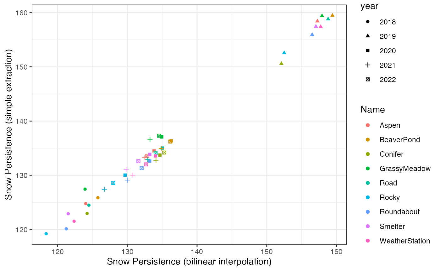 How much the extraction method matters depends on the spatial resolution
of the source data and how variable it is across space. In general, the
method matters more for coarser resolution datasets.
How much the extraction method matters depends on the spatial resolution
of the source data and how variable it is across space. In general, the
method matters more for coarser resolution datasets.
Buffered extraction at points with summaries
The above example extracts data at the exact locations of points. But
what if we want to get a sense of how the datasets vary in the landscape
surrounding the points? In this case we need to create a new polygon
dataset that covers areas within a certain distance of the points. We
can accomplish this using the st_buffer() function in the
sf package:
}
The above code creates circular polygons centered on each point with a radius of 100m. We can examine the results by plotting the original points and and the buffers on a web map:
The grey shaded areas are those covered by the buffered polygons.
We can now use these polygons to extract raster values that are
covered by the polygon areas. Since there are multiple raster cells that
fall within each polygon, we need to specify a function to use to
summarize the values of those cells for each polygon. The default is to
compute the mean value for each, but we can also specify any
R function that takes a vector for input and returns a
single value. For example, here we compute the mean, minimum, and
maximum as well as 25th and 75th percentiles of snow persistence in the
buffered areas:
snow_sample_mean <- sdp_extract_data(snow_persist_recent,
                                     vect(sites_buff100))
#> [1] "Extracting data at 9 locations for 5 raster layers."
#> [1] "Extraction complete."
snow_sample_mean$stat <- "mean"
snow_sample_min <- sdp_extract_data(snow_persist_recent,
                                    vect(sites_buff100),
                                    sum_fun="min")
#> [1] "Extracting data at 9 locations for 5 raster layers."
#> [1] "Extraction complete."
snow_sample_min$stat <- "min"
snow_sample_q25 <- sdp_extract_data(snow_persist_recent,
                                    vect(sites_buff100),
                                    sum_fun=function(x) quantile(x,probs=c(0.25)))
#> [1] "Extracting data at 9 locations for 5 raster layers."
#> [1] "Extraction complete."
snow_sample_q25$stat <- "q25"
snow_sample_q75 <- sdp_extract_data(snow_persist_recent,
                                    vect(sites_buff100),
                                    sum_fun=function(x) quantile(x,probs=c(0.75)))
#> [1] "Extracting data at 9 locations for 5 raster layers."
#> [1] "Extraction complete."
snow_sample_q75$stat <- "q75"
snow_sample_max <- sdp_extract_data(snow_persist_recent,
                                    vect(sites_buff100),
                                    sum_fun="max")
#> [1] "Extracting data at 9 locations for 5 raster layers."
#> [1] "Extraction complete."
snow_sample_max$stat <- "max"
Now that we have the extracted data, we can reshape it for visualization.
snow_sample_stats <- as.data.frame(rbind(snow_sample_min,
                           snow_sample_q25,
                           snow_sample_mean,
                           snow_sample_q75,
                           snow_sample_max))
snow_stats_long <- pivot_longer(snow_sample_stats,cols=contains("X"),
                                names_to="year",values_to="snow_persist_doy")
snow_stats_wide <- pivot_wider(snow_stats_long,names_from="stat",
                               values_from="snow_persist_doy")
snow_stats_wide$year <- gsub("X","",snow_stats_wide$year)
head(snow_stats_wide)
#> # A tibble: 6 × 9
#>     fid Name     ID year    min   q25  mean   q75   max
#>   <int> <chr> <dbl> <chr> <dbl> <dbl> <dbl> <dbl> <dbl>
#> 1     1 Rocky     1 2018   113.  117.  120.  124.  128.
#> 2     1 Rocky     1 2019   150.  153.  155.  156.  160.
#> 3     1 Rocky     1 2020   127.  129.  131.  134.  138.
#> 4     1 Rocky     1 2021   122.  126.  129.  133.  137.
#> 5     1 Rocky     1 2022   124.  127.  130.  133.  137.
#> 6     2 Aspen     2 2018   113.  117.  121.  124.  128.
The code above binds the rows of the extracted data together and then
reshapes it using the pivot_longer and
pivot_wider functions (in the tidyr package)
so that the different summaries are represented by different variables.
We can then plot the summaries of spatial variability in snow
persistence across sites and years:
library(ggplot2)
ggplot(snow_stats_wide)+
  geom_linerange(aes(x=Name,ymin=min,ymax=max,color=year),
                 linewidth=0.5,position=position_dodge(width=0.5))+
  geom_linerange(aes(x=Name,ymin=q25,ymax=q75,color=year),
                 linewidth=1.5,position=position_dodge(width=0.5))+
  geom_point(aes(x=Name,y=mean,fill=year), shape=21, color="black",size=1.5,
             position=position_dodge(width=0.5))+
  scale_y_continuous("Spring Snowpack Persistence (Day of Year)")+
  scale_x_discrete("Site")+
  theme_bw()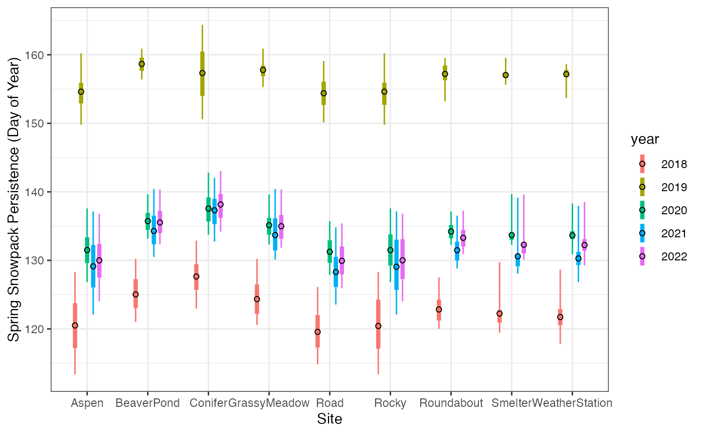
Spatial variability in spring snowpack persistence from 2018 to 2022. The thin lines span range between minimum and maximum values within 100 m of field sites, the thick lines represent the range from the 25th to 75th percentile. The open circles represent the mean.
We can see that sites melt out from seasonal snowpack in a predictable sequence, with the “Rocky”, “Road”, and “Aspen” sites usually the first to melt, and the others usually later. We can also see the tremendous variability between years, with sites in 2018 melting more than 3 weeks earlier than in 2019.
We can also see that the late-melting year (2019) shows reduced variability in melt timing in the landscape surrounding most sites. This is evident in the smaller range between the minimum and maximum values as well as the reduced variability between sites.
Extracting summaries using lines and polygons
The example above creates polygons buffering field sites represented by points, but we can also summarise data products using other polygon and vector data. The example below reads in a polygon representing the Gothic Townsite area and computes summaries of snow dissapearance across the entire polygon:
## Reads in polygons
gt_poly <- vect(st_read("https://rmbl-sdp.s3.us-east-2.amazonaws.com/data_products/supplemental/GT_region_vect_1m.geojson"))
#> Reading layer `GT_region_vect_1m' from data source
#>   `https://rmbl-sdp.s3.us-east-2.amazonaws.com/data_products/supplemental/GT_region_vect_1m.geojson'
#>   using driver `GeoJSON'
#> Simple feature collection with 1 feature and 2 fields
#> Geometry type: POLYGON
#> Dimension:     XY
#> Bounding box:  xmin: 327105 ymin: 4313359 xmax: 328312 ymax: 4314793
#> Projected CRS: WGS 84 / UTM zone 13N

## Extracts summaries
snow_gt_mean <- sdp_extract_data(snow_persist_recent,gt_poly)
#> [1] "Extracting data at 1 locations for 5 raster layers."
#> [1] "Extraction complete."
snow_gt_mean$stat <- "mean"
snow_gt_min <- sdp_extract_data(snow_persist_recent,gt_poly,
                                    sum_fun="min")
#> [1] "Extracting data at 1 locations for 5 raster layers."
#> [1] "Extraction complete."
snow_gt_min$stat <- "min"
snow_gt_q10 <- sdp_extract_data(snow_persist_recent,gt_poly,
                                    sum_fun=function(x) quantile(x,probs=c(0.1)))
#> [1] "Extracting data at 1 locations for 5 raster layers."
#> [1] "Extraction complete."
snow_gt_q10$stat <- "q10"
snow_gt_q90 <- sdp_extract_data(snow_persist_recent,gt_poly,
                                    sum_fun=function(x) quantile(x,probs=c(0.9)))
#> [1] "Extracting data at 1 locations for 5 raster layers."
#> [1] "Extraction complete."
snow_gt_q90$stat <- "q90"
snow_gt_max <- sdp_extract_data(snow_persist_recent,gt_poly,
                                    sum_fun="max")
#> [1] "Extracting data at 1 locations for 5 raster layers."
#> [1] "Extraction complete."
snow_gt_max$stat <- "max"

## Binds output together
snow_gt_stats <- as.data.frame(rbind(snow_gt_min,
                                    snow_gt_q10,
                                    snow_gt_mean,
                                    snow_gt_q90,
                                    snow_gt_max))

## Reshapes for plotting.
snow_gt_long <- tidyr::pivot_longer(snow_gt_stats,cols=contains("X"),
                                names_to="year",values_to="snow_persist_doy")
snow_gt_wide <- tidyr::pivot_wider(snow_gt_long,names_from="stat",values_from="snow_persist_doy")
snow_gt_wide$year <- gsub("X","",snow_gt_wide$year)

## Plots variability.
ggplot(snow_gt_wide)+
  geom_linerange(aes(x=year,ymin=min,ymax=max,color=year),
                 linewidth=0.5,position=position_dodge(width=0.5))+
  geom_linerange(aes(x=year,ymin=q10,ymax=q90,color=year),
                 linewidth=1.5,position=position_dodge(width=0.5))+
  geom_point(aes(x=year,y=mean,fill=year), shape=21, color="black",size=1.5,
             position=position_dodge(width=0.5))+
  scale_y_continuous("Spring Snowpack Persistence (Day of Year)")+
  scale_x_discrete("year")+
  theme_bw()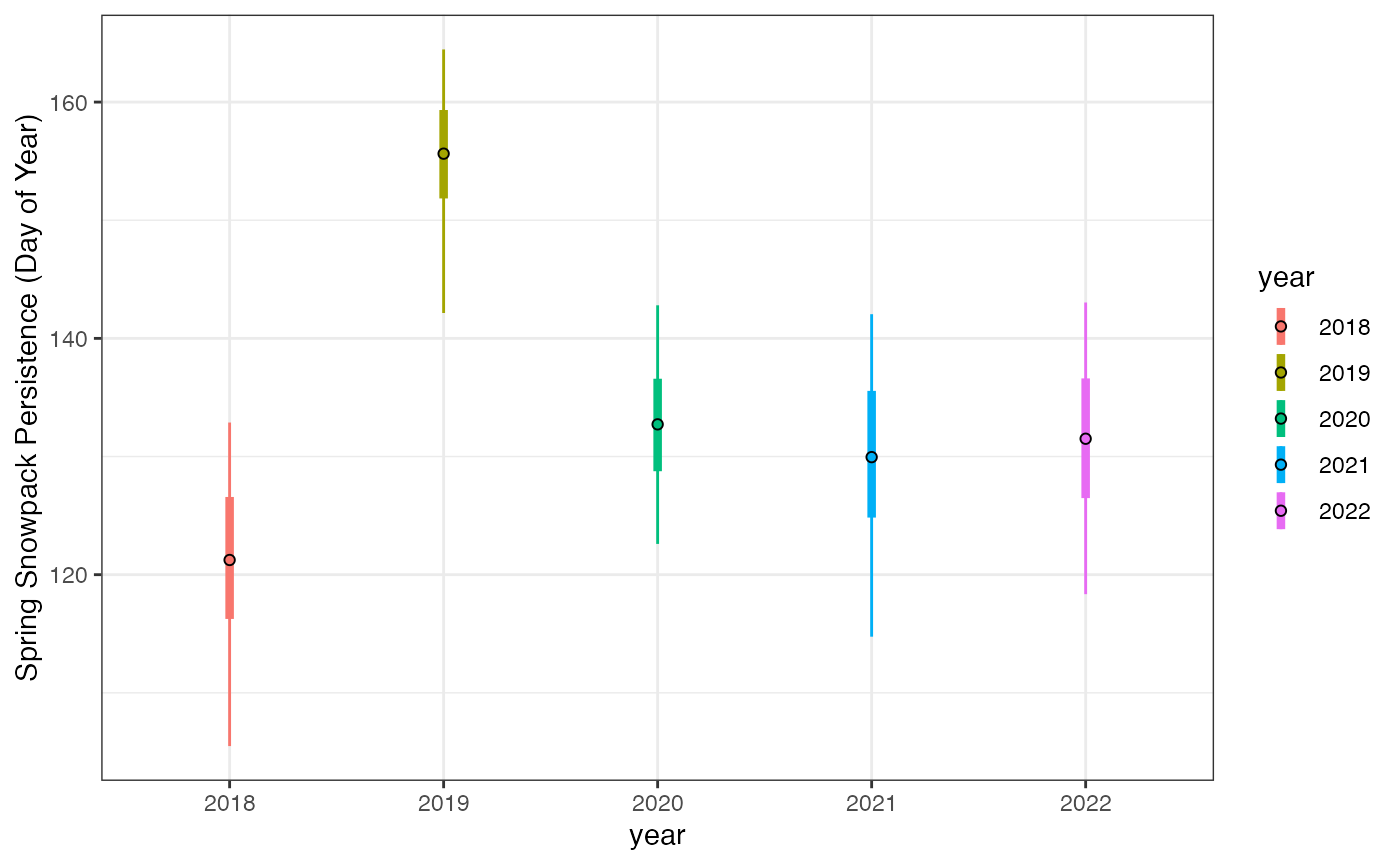
Summarising categorical data products
The strategies above work well for summarising data products that represent continuous numeric values, but categorical rasters such as land cover maps pose an additional challenge. Most summary functions that make sense for continuous data (e.g. mean, median, max) do not make sense for categorical data.
As an example, we can load a landcover map for the vicinity of the Gothic Townsite polygon we loaded above.
ug_lc <- sdp_get_raster("R3D018")
lc_crop <- crop(ug_lc,st_bbox(gt_poly))
plot(lc_crop,main="Gothic Landcover")
plot(gt_poly,add=TRUE)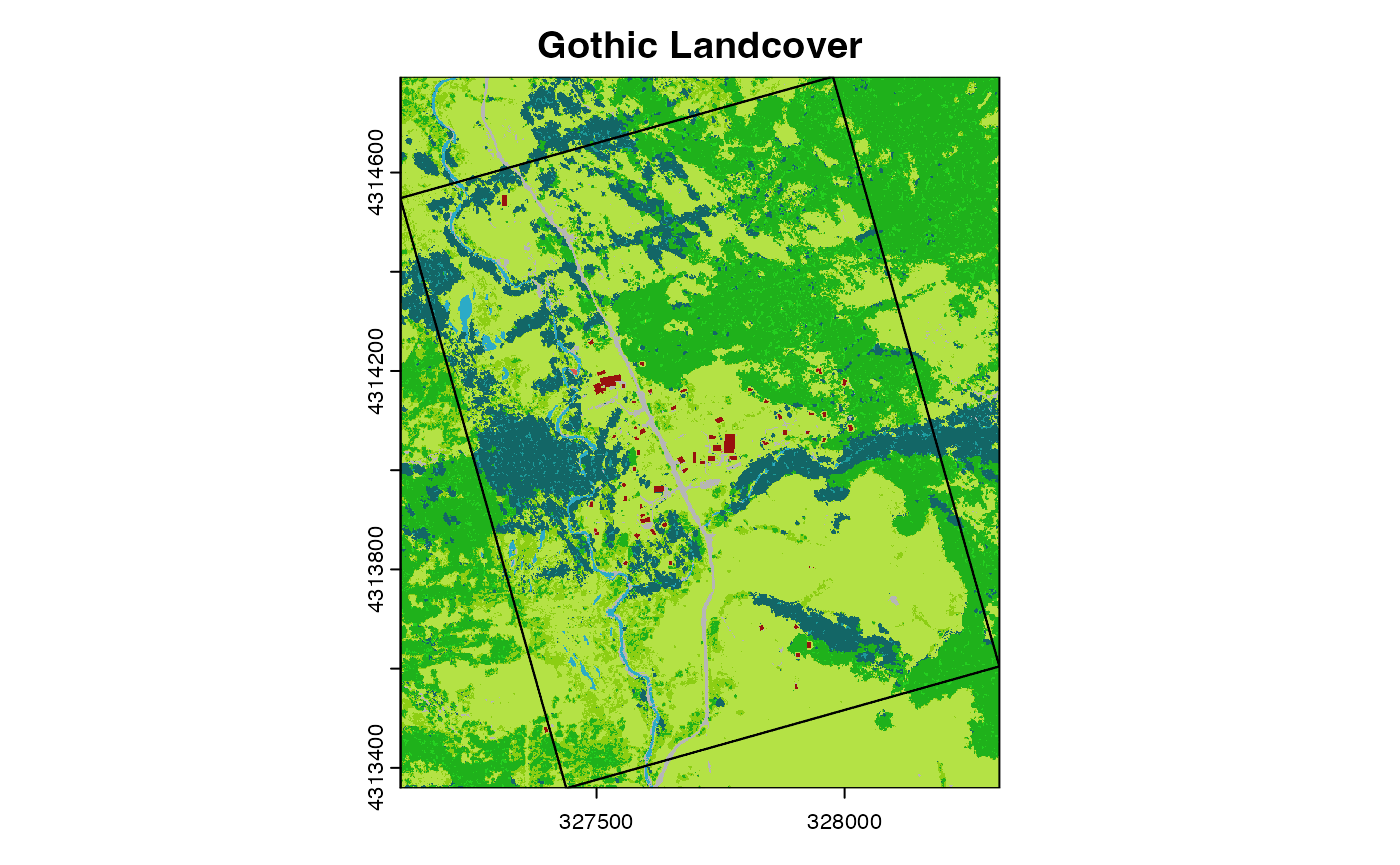 What if we want to estimate what proportion of the study area is covered
by each landcover class? In this case, we want to extract all the raster
values within the polygon and then summarise them. We can accomplish
this using a combination of the
What if we want to estimate what proportion of the study area is covered
by each landcover class? In this case, we want to extract all the raster
values within the polygon and then summarise them. We can accomplish
this using a combination of the sdp_extract_data() function
along with the group_by() and summarise()
functions in the dplyr package:
gt_lc_all <- sdp_extract_data(lc_crop,gt_poly,bind=FALSE,return_type="DataFrame",
                              sum_fun=NULL,weights=TRUE)
#> [1] "Extracting data at 1 locations for 1 raster layers."
#>
|---------|---------|---------|---------|
=========================================

[1] "Extraction complete."
str(gt_lc_all)
#> 'data.frame':    1119828 obs. of  3 variables:
#>  $ ID                : num  1 1 1 1 1 1 1 1 1 1 ...
#>  $ UG_landcover_1m_v4: num  2 2 2 2 2 2 2 2 2 2 ...
#>  $ weight            : num  1 1 1 1 1 ...
When we specify sum_fun=NULL in the
sdp_extract_data() function above, the function returns a
data frame with all of the (~1.1 million) cell values that intersect the
polygon. By specifying weights=TRUE we also return the
proportion of each raster cell that is covered by the polygon. If cells
along the boundary of the polygon are partially covered, then their
weight in the resulting data will be less than one.
Now we can summarise these values for each landcover class:
library(dplyr)
#>
#> Attaching package: 'dplyr'
#> The following objects are masked from 'package:terra':
#>
#>     intersect, union
#> The following objects are masked from 'package:stats':
#>
#>     filter, lag
#> The following objects are masked from 'package:base':
#>
#>     intersect, setdiff, setequal, union
gt_area <- st_area(st_as_sf(gt_poly))
cell_size <- res(lc_crop)

gt_lc_sum <- gt_lc_all %>%
            group_by(UG_landcover_1m_v4) %>%
            summarise(n_cells=sum(weight),
                      covertype_area=n_cells*cell_size[1],
                      covertype_prop=covertype_area/gt_area)
gt_lc_sum
#> # A tibble: 10 × 4
#>    UG_landcover_1m_v4 n_cells covertype_area covertype_prop
#>                 <dbl>   <dbl>          <dbl>        [1/m^2]
#>  1                  1 166899.        166899.       0.149
#>  2                  2 265807.        265807.       0.237
#>  3                  3 502699.        502699.       0.449
#>  4                  4  13624.         13624.       0.0122
#>  5                  6  20291.         20291.       0.0181
#>  6                  7   6283.          6283.       0.00561
#>  7                  8    269.           269.       0.000240
#>  8                 10 113793.        113793.       0.102
#>  9                 11   8944.          8944.       0.00799
#> 10                 12  21219.         21219.       0.0189
Now we’ve got an estimate of the area and proportion of each landcover class in the polygon. The classes have numeric codes, but we can match these with the names of the landcover classes from the metadata:
lc_meta <- sdp_get_metadata("R3D018")
lc_codes <- 1:12
lc_classes<- c("evergreen trees and shrubs",
             "deciduous trees greater than 2m tall",
             "meadow, grassland and subshrub",
             "persistent open water",
             "persistent snow and ice",
             "rock, bare soil, and sparse vegetation",
             "building or structure",
             "paved or other impervious surface",
             "irrigated pasture and other cultivated lands",
             "deciduous shrubs up to 2m tall",
             "evergreen forest understory and small gap",
             "deciduous forest understory and small gap")
lc_df <- data.frame(UG_landcover_1m_v4=lc_codes,
                    class_name=lc_classes)
gt_lc_names <- left_join(gt_lc_sum,lc_df,by="UG_landcover_1m_v4")
gt_lc_names[,-1]
#> # A tibble: 10 × 4
#>    n_cells covertype_area covertype_prop class_name
#>      <dbl>          <dbl>        [1/m^2] <chr>
#>  1 166899.        166899.       0.149    evergreen trees and shrubs
#>  2 265807.        265807.       0.237    deciduous trees greater than 2m tall
#>  3 502699.        502699.       0.449    meadow, grassland and subshrub
#>  4  13624.         13624.       0.0122   persistent open water
#>  5  20291.         20291.       0.0181   rock, bare soil, and sparse vegetation
#>  6   6283.          6283.       0.00561  building or structure
#>  7    269.           269.       0.000240 paved or other impervious surface
#>  8 113793.        113793.       0.102    deciduous shrubs up to 2m tall
#>  9   8944.          8944.       0.00799  evergreen forest understory and small …
#> 10  21219.         21219.       0.0189   deciduous forest understory and small …
Success! Although this example uses a single polygon, a similar workflow would work for datasets that contain multiple polygons as well as line data.
Strategies for boosting performance
In the examples above, we have limited the amount of data that we need to download locally by connecting to data products stored on the cloud. For many use cases, this is great, but sometimes these operations can be quite slow, and are often limited by the speed of your internet connection.
Below are a few strategies for speeding up extracting data for large rasters, rasters with lots of layers, and / or large numbers of field sites:
Downloading raster data locally
The default behavior of sdp_get_raster() is to connect
to a cloud-based data source without downloading the file(s) locally. If
an extraction operation is prohibitively slow, sometimes it makes sense
to download the files locally before running
sdp_extract_data().
To download the files, you need to specify
download_files=TRUE and then a local file path for storing
the files:
snow_persist_local <- sdp_get_raster("R4D001", years = c(2018:2022), download_files = TRUE,
                                     download_path = "~/Downloads",overwrite=FALSE)
#> [1] "Returning yearly dataset with 5 layers..."
#> [1] "All files exist locally. Specify `overwrite=TRUE` to overwrite existing files."
#> [1] "Loading raster from local paths."
With the default argument overwrite=FALSE the function
will download files for any layers that don’t already exist in the local
filesystem and then create a SpatRaster object that is
linked to the local datasource instead of the cloud. If all of the files
already exist locally, then no files will be downloaded. This means that
after the initial download step, subsequent calls to
sdp_get_raster() that reference those same files (or
subsets of those files) will not result in additional downloads.
Specifying overwrite=TRUE will cause datasets to be
re-downloaded each time the function is run.
We can look at the speedup conferred by local downloads for large
extraction operations. The function spatSample() in the
terra package generates (potentially large) random or
regular samples of raster cells. Here we use this function to compare
the speed of extractions on cloud-based and local datasets:
# Cloud-based dataset
start <- Sys.time()
sample_cloud <- spatSample(snow_persist_recent,size=100,method="random")
Sys.time() - start
#> Time difference of 41.10631 secs

# Local dataset.
start <- Sys.time()
sample_local <- spatSample(snow_persist_local,size=100,method="random")
Sys.time() - start
#> Time difference of 0.440625 secs
If the datasets already exist locally, then the operation is much faster. Obviously this doesn’t take into consideration the amount of time it takes to download the files initially.
Crop then extract
Another strategy is effective when the sites to sample or extract data cover a small portion of the extent of the full raster. In this case, it can be more efficient to crop the raster to the extent of the sites before performing the extraction. Cropping a cloud-based dataset will download only the cropped subset of the data desired.
As an example of this strategy, we will generate a large number of random points within the boundary of the Gothic Townsite polygon we loaded earlier, and then crop a large elevation dataset to the extent of the raster.
gt_pts <- spatSample(gt_poly,size=1000)
dem <- sdp_get_raster("R3D008")
dem_crop <- crop(dem,gt_pts)
ncell(dem_crop)
#> [1] 1616643
c("ncells_full"=ncell(dem),"ncells_cropped"=ncell(dem_crop))
#>    ncells_full ncells_cropped
#>     6026339412        1616643
The much smaller cropped dataset is now stored in memory locally, so now subsequent operations will be very fast.
start <- Sys.time()
elev_extract_full <- sdp_extract_data(dem,locations=gt_pts)
#> [1] "Extracting data at 1000 locations for 1 raster layers."
#> [1] "Extraction complete."
Sys.time() - start
#> Time difference of 6.519675 secs

start <- Sys.time()
elev_extract_cropped <- sdp_extract_data(dem_crop,locations=gt_pts)
#> [1] "Extracting data at 1000 locations for 1 raster layers."
#> [1] "Extraction complete."
Sys.time() - start
#> Time difference of 0.01676106 secs
Parallel processing
For extraction operations that get data from a large number of layers
(such as daily climate time-series), it can make sense to do the
extraction in parallel across multiple R processes. The
foreach and doParallel packages provide
facilities for setting up this kind of parallel process. The core of
this workflow is a call to the function foreach, which is
similar to a standard for loop, but allows different
iterations of the loop to be sent to independent R processes.
A complication with parallel processing for this use case is that
it’s currently not possible to pass SpatVector or
SpatRaster objects between the parent R process and the
parallel worker processes. This means that we need to create separate
SpatRaster objects for subsets of data to be processed in
parallel.
Here’s an example of parallel extraction of daily air temperature time-series for the small number of research sites we worked with earlier:
library(foreach)
library(doParallel)
#> Loading required package: iterators
#> Loading required package: parallel

## Can't pass SpatVector or SpatRaster objects via Foreach, so convert to sf.
locations_sf <- st_as_sf(sites_proj)

## Sets the number of parallel processes.
n_workers <- 4

start <- Sys.time()
cl <- makeCluster(n_workers)
registerDoParallel(cl)
days <- seq(as.Date("2016-10-01"),as.Date("2022-9-30"), by="month")

extr_list <- foreach(i=1:length(days),.packages=c("terra","rSDP","sf")) %dopar% {
  tmax <- sdp_get_raster("R4D007",date_start=days[i],
                         date_end=days[i],verbose=FALSE)
   locations_sv <- vect(locations_sf)
   extr_dat <- sdp_extract_data(tmax,locations=locations_sv,
                                verbose=FALSE,return_type="sf")[,4]
   (st_drop_geometry(extr_dat))
}
stopCluster(cl)
tmax_extr <- cbind(locations_sf,
                   do.call(cbind,extr_list))
elapsed <- Sys.time() - start
elapsed
#> Time difference of 43.39494 secs
Finally we can reshape the data for visualization.
tmax_extr_long <- pivot_longer(tmax_extr,cols=contains("X"),
values_to="average_tmax",
names_to="year_month")
tmax_extr_long$date <- as.Date(paste0(gsub("X","",tmax_extr_long$year_month),".15"),
format="%Y.%m.%d")
ggplot(tmax_extr_long)+
geom_line(aes(x=date,y=average_tmax,color=Name))+
scale_y_continuous("Average Monthly Tmax (C)")+
theme_bw()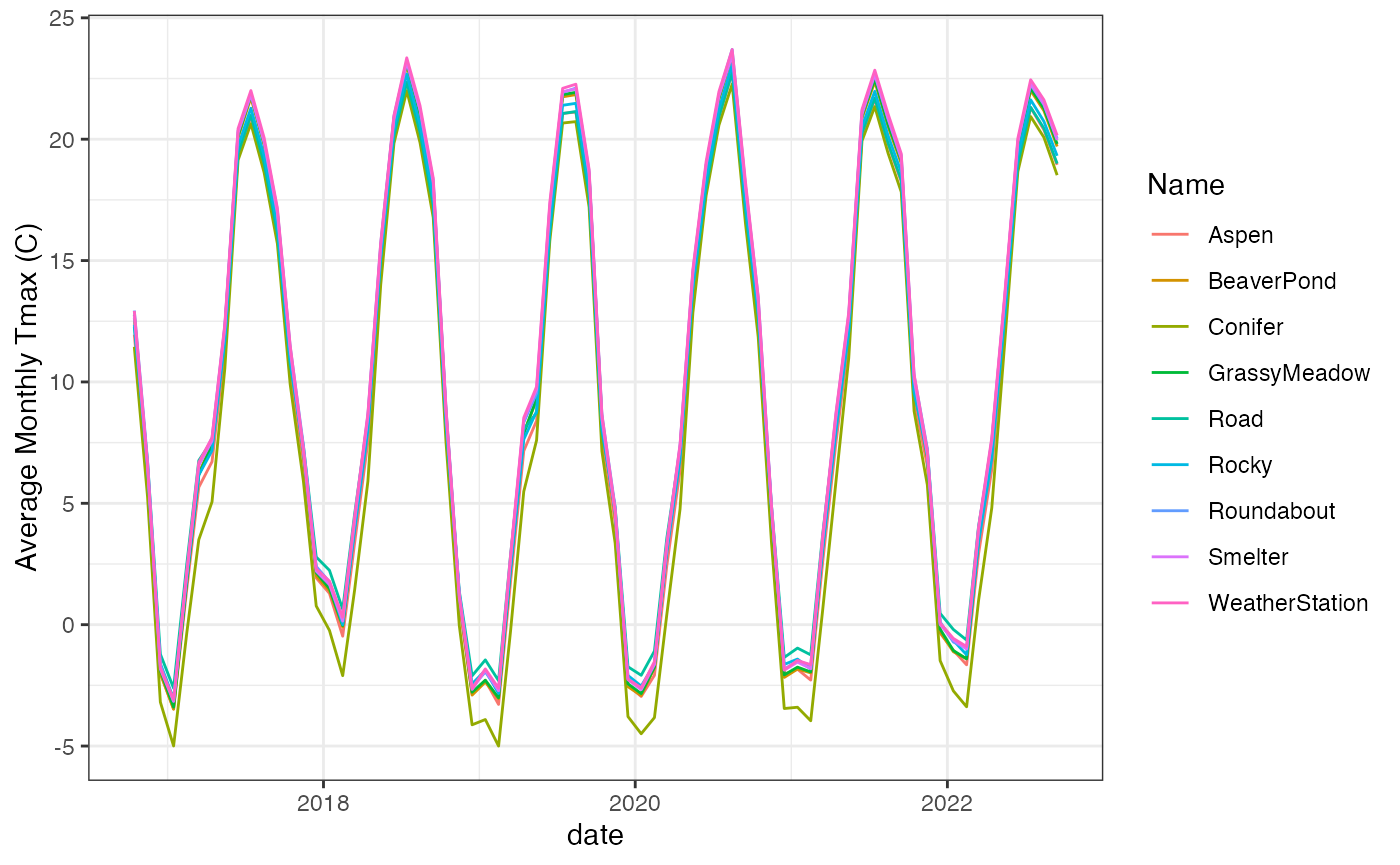 These sites are all within a few hundred meters of each other so
differences in microclimate are mostly due to vegetation structure and
solar radiation.
These sites are all within a few hundred meters of each other so
differences in microclimate are mostly due to vegetation structure and
solar radiation.